CMRA Surveys Market Risk Reporting Techniques

Last year, the Securities and Exchange Commission announced it would allow companies to choose between three different methods to fulfill market risk disclosure requirements. Derivatives users could choose between tables of individual risk factor data, sensitivity analyses or value-at-risk-type information.

Which method will companies be using to fulfill these requirements? According to a January 1998 survey of some 30 financial firms and corporations by Capital Market Risk Advisors, 80 percent of the respondents indicated their disclosure methods would involve techniques similar to those they already use for internal risk measurement and reporting.

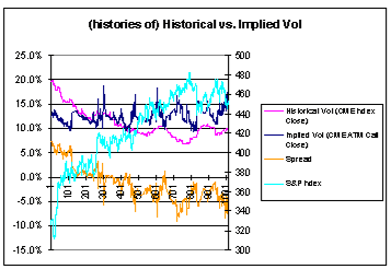
Most banks and broker-dealers already use value-at-risk internally to measure the risk of their trading activities, and most of these plan to use VAR to disclose the market risk of trading activities to the SEC, though they may not use VAR in disclosing nontrading activities.

The majority of insurance companies surveyed, meanwhile, use sensitivity analysis to meet regulatory reporting requirements, and most of these plan to use the technique to meet SEC requirements.

By contrast, most of the smaller firms that do not currently use VAR plan to use tables of individual risk factor data to comply with the SEC requirements.

The survey discovered a number of interesting VAR-related factoids:

• The length of the observation period used in the calculations will range from less than one year to more than three years.
• The amount of VAR generally represented less than 1 percent of the respondents’ book values among broker-dealers and banks that offered their 1997 statistics.
• More than 90 percent of these plan to use VAR calculations for pricing models rather than for concrete changes in earnings, values or cash flows.
• The most common model is the analytic variance-covariance VAR, with aproximately 50 percent selecting this method by itself. Most cited the less computationally intensive nature of this calculation relative to historical VAR (20 percent of respondents), Monte Carlo-based VAR (25 percent) or other stimulation methods (5 percent).
• Twenty percent of the VAR-using firms ignore nonlinearity positions altogether, while 25 percent of the respondents made adjustments for option holdings by measuring the delta of their positions. Another 30 percent made adjustments using both delta and gamma.
• In general, those firms using VAR take into account the correlation effects across risk exposures both within and across instrument types. For about 90 percent of the respondents, use of empirical correlations is the preferred methodology.
• All of the bank and broker-dealer respondents plan to use a one-day holding period, while insurance companies and corporates plan to use periods of two weeks to one year.
• Of the firms that plan to use sensitivity analysis, all plan to use actual, observed fair values rather than pricing model computations. Unlike the VAR-using firms that account for volatility and correlation, sensitivity analysis-using firms plan to show the sensitivity only to price changes and market factors such as currency rate or interest rate changes.

CMRA Surveys Market Risk Reporting Techniques

Rogue Trading Insurance

The Titanic, Bruce Springsteen’s voice, NASA satellites and countless other odd and famous objects have been insured by Lloyds of London contracts over the years. Now, in an effort to protect customers from the Nick Leesons of the world, the venerable institution has begun offering insurance against rogue traders.

While other insurers offer policies to cover trading, they define fraudulent trading as breaking rules either to cause losses or for personal financial gain—in other words, stealing. In Leeson’s case, however, Barings was not protected by its fidelity trading insurance because Leeson exceeded position limits not to bolster his commissions but to cover his earlier losses. The new Lloyds policies also cover unauthorized trading undertaken merely to get out of trading holes.

The policies, written by SVB Syndicates, a Lloyds subsidiary dedicated to specialty coverage of financial institutions, provide up to $300 million to cover direct financial loss caused by unauthorized, concealed or falsely recorded trading by any person trading for the insured institution.

“What we found when we looked at the losses in unauthorized trading was that quite typically they did not include dishonesty,” says Steven Burnhope, director of SVB. “It was often an action taken [simply] to make a profit. Our customers said to us that, with the emergence of trading as a major component of their earnings these days, the traditional products didn’t address the risks that were emerging in those areas.”

While SVB’s new policies cover only proprietary trading activities, another Lloyds subsidiary, Stone Financial Risks, is now offering policies geared toward securities brokers as well, offering protection for losses caused by dealers’ clients.

The annual premiums for the rogue trading policies will range between $2 million and $10 million, with annual deductibles of between $10 million and $25 million, to be determined on a case-by-case basis. SBC and Stone will examine each firm’s internal risk management framework, making sure that solid trading controls are in place. Neither plans to issue policies to firms that fail to meet the basic requirements. In January, Chase purchased the first policy, and some 40 other financial institutions have asked for quotations thus far. Since Lloyds represents 60 of the world’s 100 largest banks, it hopes that the policies will take off.

“We didn’t know at the beginning if we would be able to provide cover in this area,” says Burnhope, “because it is one that insurers have found quite difficult to assimilate.” It is clear now, however, that with these policies another level of risk management tool has emerged. Is reinsurance of rogue trading policies far off?

Rogue Trading Insurance

The Post Bashes Morgan

The New York Post is not normally the first place you'd turn for articles about RiskMetrics. On March 8, however, columnist John Dizard mocked Morgan’s risk management systems for failing to predict the $587 million fourth quarter earnings loss the bank holding company designated as “nonperforming assets, primarily swaps.”

The problem, claims Dizard, goes to the heart of the bank's ability to control risk. Instead of chasing the retail credit card businesses like other banks, he explains, Morgan decided to take the less traveled road and become a global derivatives player. “There was, however, a reason that this road was less traveled by—it was studded with land mines.”

RiskMetrics, he says “uses the same probability theory analysis that a serious gambler would employ in estimating his risk/reward ratio—Morgan may have ordered RiskMetrics from the same Acme Co. that used to supply Wile E. Coyote with those rocket-powered roller skates.”

He goes on to quote an unnamed source on the merger rumors swirling around the bank. “I think of them as pink, trembling aristocrats worrying about how their cruel new barbarian masters will use them,” says the source. “They want to be rescued by someone like Deutsche Bank, but Deutsche doesn't need the name. Someone with a lot of money and not so much class will move in.” By now everyone has heard that 1997 was a record year for most major options exchanges. But many would be surprised to learn that much of that growth was fueled by individual stock options, as opposed to index options, despite the success of new listed index products such as the Chicago Board Options Exchange’s options on the Dow Jones Industrial Average.

How to explain the relative success of equity options? Let Goldman Sachs count the ways. In two recent research reports, “U.S. Stock Options Move to Center Stage: A Look Behind the Scenes,” and “Relative Value in U.S. Stock vs. Index Options: Is Dispersion Cheap?” Goldman researchers explain why equity options have soared, and what investors should do about it.

In the past three years, stock option activity has increased at an annual rate of more than 20 percent. A number of developments point to continued success of equity options. The growth of hedge funds with a stock focus, in which managers use stock options to leverage equity views and to implement bearish views with more precision than index options, has had a profound effect. In addition, a more subdued equity market, which Goldman believes is in the offing, should place additional emphasis on stock selection more than overall market performance. There has also been an increased desire on the part of wealthy investors to hedge the capital gains they have realized in concentrated stock funds, and an increasing prevalence of stock options in employee compensation structures, which increases general familiarity of equity option products. The bustling long-term equity anticipation securities (LEAPS) market has contributed as well, allowing investors to take longer views on particular equities.

The report also points to an increasingly beneficial regulatory environment, including wider position limits for those using the equity hedge exemption, the removal of position limits on equity FLEX options and the Securities and Exchange Commission’s move to model-based capital requirements for listed broker-dealers.

In addition, changes to the tax law, such as the elimination of the short-short rule, have made options more tax-advantageous to investors. Goldman also argues that there has been an increasing acceptance of derivatives in the financial world, and that an increase in corporate restructurings has enticed many investors to use options to speculate on potential merger and acquisition activity.

As if that weren’t enough, Goldman asserts that the volume of calls as a percentage of total volume has hovered around 70 percent for equity options, whereas it has struggled to reach 50 percent for index options. This indicates that while investors use equity options for leveraged investments, they use index options primarily to hedge their broad-based exposures. “In light of the strong U.S. equity market returns in the last few years,” says Goldman, “such index option strategies may have fallen in the shadows…As growth of the U.S. market slows to a more ‘normal’ pace [this year], stock selection and sector rotation are likely to become of increased importance.”

But how can investors capitalize on this trend? Goldman notes that “the spread of stock option to index option volatility was in a general trend of widening during the early 1990s as implied index volatility fell sharply and stock option volatility was stable. Since mid-1994, however, the spread has narrowed and may now be poised to begin another multiple-year rising trend as bottom-up forces that emphasize stock selection gain in relative importance.” Further, correlation is poised to decrease, says Goldman, so stock option strategies are preferable to index option strategies “to capture any increase in the dispersion across stock returns.” With this in mind, Goldman offers three possible strategies for investors:

• Favor option positions that are long volatility on extremely attractive or unattractive stocks. Replace or augment stock positions with call options or call spreads (long at-the-money call/short out-of-the-money call) as a way of capturing the upside of value-added stock selection while limiting downside exposure.
• In buying stock options vs. sector options, be sensitive to sectors where innovation or market developments shift the returns across participants dramatically, as in technology and consumer nondurables, where competition is intense.
• Favor short or neutral volatility positions in index options for risk management by selling out-of-the-money call options at target index levels or using long put/short call strategies for downside hedging.

The Post Bashes Morgan

Prepackaged Volatility Plays (vol. 1)

Two new products hope to make volatility trading a no-brainer.

All derivatives traders know that option prices really boil down to the market’s expectation of the future volatility of the underlying instrument, because all the other determinants of an option’s price—the underlying price, time to maturity, interest rate and strike price—are objective. Volatility is the X factor, and only rarely does an option’s actual, realized volatility replicate the implied volatility reflected in its valuation.

Traders typically hedge implied volatility by constructing elaborate—and often highly expensive—series of short and long straddles based on differing strike prices, styles and expirations. Although over-the-counter volatility structures have been offered for years, they have been highly illiquid and do not offer price transparency—characteristics sure to scare off traders.

Now volatility traders will have a much easier time of it, thanks to two new products released in January: volatility futures from the Deutsche Terminborse and volatility swaps from Salomon Smith Barney.

The DTB became the first exchange in the world to list volatility futures based on an underlying index of implied volatility when it launched the VOLAX future on January 19. The VOLAX is based on the implied volatility of its DAX index options, which is represented by the VDAX, a set of eight volatility indices introduced by the DTB last summer.

VOLAX futures allow traders of DAX options the ability to manage their volatility risk in a single instrument. “There are certain traders in the market who play with volatilities to trade volatility strategies,” says Elmar Werner, product developer at the DTB. “It is much easier for them to use the VOLAX instead of a combination of DAX options. It’s cheaper in terms of the exchange fees, and you don’t have to look for the combinations. It’s a single product that’s more efficient and easier to use.”

VOLAX futures have a number of other uses as well, including hedging warrant issues; eliminating the vega component (the change in an option’s price caused by changes in volatility) upon the creation of delta (the degree of change in an option’s premium, based on changes in the underlying) or gamma (the rate of change of delta) positions; and facilitating the buying or selling of options upon extremely high or low volatilities for DAX option market makers who are obliged to make binding quotes. The instruments can also be used to speculate on rising or falling volatilities, to exploit mispricings across the DAX option volatility curve, to arbitrage against DAX options, and to serve as the underlying for warrants. (See box.)

But what about traders who aren’t exposed to the DAX but want to hedge their volatility risk? Salomon Smith Barney thinks it has the answer for them. In January the firm began promoting volatility swaps, a product meant to appeal to traders who want to hedge their volatility exposures without constructing elaborate and unwieldy positions—and who thus want to escape bid-offer spreads, commissions, clearing costs and the various trade-support costs that the listed markets reap.

Volatility swaps are traded as follows: Salomon Smith Barney enters into an OTC agreement with a counterparty. At maturity, the value of the swap depends only on the realized volatility of the asset, and not the volatility path the asset has taken during the life of the trade, which can sometimes make for higher costs in traditional listed volatility structures. The investor merely contracts with Salomon Smith Barney, which either buys or sells an option portfolio, delta hedges the portfolio and pays the customers the positive return or collects the negative return. Salomon takes care of all the operational costs, including risk management, systems, traders, back office and clearing.

Volatility swaps have several applications. Customers can sell swaps on the one-year volatility of the Standard & Poor’s 500, an attractive proposition for those who don’t expect the market to crash in the next 12 months. The S&P one-year volatility is currently trading around 25 percent, even though realized one-year volatility has rarely exceeded 18 percent, largely as a result of investor nervousness. Corporates can short individual stock volatility to hedge their volatility exposures when planning to issue convertible bonds. According to Salomon, “if volatility were to decline, the higher coupon the company would have to pay would be offset by the positive value of the swap at maturity…[while] if the volatility were to increase, the convertible to be issued would be more valuable…[so] the company could pay a lower coupon.”

Many funds have positions in Japanese converts and warrants, leaving them long volatility of individual stocks. Since there are no listed option markets in Japan for equities, shorting some stocks can be difficult. Salomon’s new swap products allow investors to hedge their long volatility positions in Japanese equities by selling one-year or even two-year Nikkei volatility to Salomon. In addition, index funds can use Salomon volatility swaps to reduce the amount of tracking error that could attend massive increases in market volatility.

Some have predicted that volatility will become the next big asset class. Salomon and DTB certainly hope that’s the case more rather than less, sooner rather than later.

Arbing the VOLAX
The VOLAX could present tremendous arbitrage profit possibilities if it is mis-priced early on. According to the DTB, by constructing a “replication portfolio” of the VOLAX, traders can arbitrage overvalued VOLAX futures relatively easily. For example, say the fair price of the VOLAX is DM 1,575, but the VOLAX is traded at DM 1,600—an arbitrage window of DM 25. To arbitrage 100 VOLAX futures, a replication portfolio consisting of 102 long straddles expiring at Tl and 80 short straddles expiring at Ts is constructed, paid for by borrowing from the money market. The delta of the replication portfolio is 19.72, far below that of a DAX future. At Tl, the VOLAX is no longer mispriced, so the arbitrage window closes. The forward volatility at Tl has risen to 16.25 percent, and the DAX has fallen by 50 points, so the VOLAX is now traded at DM 1625. Buying back 100 VOLAX futures therefore results in a loss of DM 2,500, but this is divided into the loss resulting from the change in fair futures price, which is DM 5,000. The result: a profit of DM 2,500.
—Source: Deutsche Terminborse

Prepackaged Volatility Plays

Historical Volatility vs. Implied Volatility Strategies

Historical Volatility vs. Implied Volatility Strategies - Part 1

Please note, as ART Consulting/Research is a fee based service, in the following the results have been "sanitised" to disguise the specific markets, trading factors, strategy parameters and many other essentials. Of course, all of the analyses is based on real market conditions and real world trading considerations (trans cost, funding, etc). For access to the "un-sanitised" results, and for analysis tailored to your needs please submit an email via Request More Information.

One particularly compelling aspect of options trading is the question of the relationship between historical volatility (vH) and implied volatility (vI), if any. Many traders have a sense that there might be some connection between these two measures that could be helpful in forecasting or trading. This is a complex matter, and the first step (and so this "the Part 1") is to discover if there are possibilities for improving the P&L based on such considerations (i.e. "is there any chance at all of making money with this approach?").

• Can this be modelled?
• Can this be (predictably) exploited for profit?
• Can this be done consistently, and with sufficiently high risk-adjusted returns to warrant assignment of capital, limits, salaries, etc.

This area is particularly tricky in part due to the complications both of understanding and modelling volatility, and that of the coupled complications of assessing the correct or best trading strategy to exploit any potential benefit from such relationships.

1. Modelling Considerations: notice that options models are required for both valuation and rebalancing calculations for any trading strategy aiming to profit from a vH vs. vI. There are many such issues to consider. For example, there is no guarantee that an empirical measure such as vH is consistent with the measure vI assumed in a theoretical model such Black-Scholes (see TG2RM1st Chapters 8-12 for the "mountain range" metaphor for theoretical uncertainty vs. reality and P&L impact). Another consideration is that empirical measures necessarily measure the past, while implied measures (partially) reflect expectations about the future. For these and many other reasons, just arriving at a suitable and practical level of "relationship assessment" is a very complex process.
2. Trading Strategy Considerations: The modelling considerations may or may not be performed independently from trading strategy assumptions. Assume for a moment that those relationships exist (a very big assumption). Now, there is still the matter of assessing the actual trading strategy for the (risk-adjusted) P&L performance. In options trading, the strategies to exploit such relationships almost always rely on dynamic/synthetic replication. This means that the holding period rebalancing sequence of trades (i.e. the strategy) will vary depending on how the volatility relationships above are expressed. Adding to the complications is the observation that options position cannot isolate volatility, and so there will be other effects to contend with (e.g. at least the usual Greeks etc.). This means that the strategy consideration and the resultant risk-adjusted P&L's will require very careful interpretation. For example, a high frequency rebalance Delta neutral vanilla call option strategy's P&L may or may not be directly comparable to a Delta/Vega neutral straddle strategy given certain specific issues in the nature of any volatility relationships determined in step 1) above.

The first step is to determine if there is any hope of a P&L advantage at all. If such exists, then more resources might be committed for further analysis or trading. One answer to this question follows from a PaR analysis of various (vH vs. vI) relationships combined with various trading strategies.

As always, PaR analysis with the Pr/rO ® software employs very realistic holding period forward and backward simulations of market scenarios and trading strategies (including all of the usual nitty gritties faced by traders doing real trading, such as transactions costs, funding, liquidity constraints, credit, etc ... ). Other examples of PaR analysis are provided in the ARBLab Samples section, such as ARBLab: P&L Optimal Options Rebalancing - 1, while all of TG2RM1st - Chapter 12 is dedicated to the introduction of PaR analysis.

A first analysis

Assume that some (vH vs. vI) relationships combined with various trading strategies have been determined. The PaR holding period net-P&L's from simulating 4,676 holding period trading strategies is shown in the figure to the right (click to ENLARGE). Each point is a net-P&L for the stated conditions. If the market pricing convention was truly arbitrage free, then the points in this graph should be distributed evenly in "three space". The "trading factors" Factor X and Factor Y are real world trading parameters as might be used by any trader but have been disguised for the purposes of this discussion. A third "trading factor" has been used for colouring the points (so, in effect this is 4-dimensional plot).

Two of the more important observations are:

1) Notice that the lower-right image shows that increasing level of Factor Y lead to consistently negative P&L's. Meaning that "doing this trade the other way around" would lead to consistently increasing P&L (though there is some asymmetry due to operating costs etc).

2) Notice that the "Colouring Factor" also shows a P&L bias. In particular, the points at the green-end of the spectrum are consistently in the negative (and so again implies that the inverse trade would be consistently profitable).

The pattern in the "dots" can be more easily seen with a surface fitting approach as in the image to the right (click to ENLARGE). This plot illustrates more clearly that increasing levels of Factor Y lead to consistent P&L bias (and so a consistently tradable condition). Using an Upper and Lower surface (in addition to other data verification methods, as is provided here), provides statistical verification of the "credibility" of the results.

The implication of this "Step 1" analysis is that there is indeed a possibility to trade "some" (vH vs. vI) relationships profitable (or at least justify further analysis).

As usual, caution is required. The analysis here, though including thousands of trades, and incorporating many real world factors cannot be taken as any perfect predictor of the future, and additional specific analysis may be required for your due diligence.

Hist Vol vs Implied Vol - Part 1

Introduction to Options Volatility

Volatility is often the most neglected of the major factors that influence option prices. But we make sure never to make that mistake when we consider possible trade recommendations. Volatility is a vitally important consideration in options trading.

Every asset has quiet periods when its options are cheap, and volatile periods when its options are expensive. Professional option traders are always aware of current volatility levels in relation to their historical context. To gain that perspective, they view historical volatility charts. The figure below shows a sample Volatility Chart for Corn:

The Volatility Chart displays two lines - one for statistical volatility (SV) and the other for implied volatility (IV). The solid SV line represents, at each point the actual volatility of the futures’ daily price volatility. Statistical volatility is often referred to as “historical” volatility, but many prefer the term statistical since volatility charts contain historical data for both SV and IV. The dashed IV line represents, at each point, the average implied volatility for the futures.

In other words, the SV line shows you the actual volatility of the futures, while the IV line shows you the volatility implied by the prices of the options of that futures. They should normally be fairly close together. If they are not, it would indicate the price of the options is not reflecting the actual volatility of the futures. At the bottom of the chart is a table that summarizes the average SV and IV for various time periods.

Volatility Charts are also useful for determining what “normal” volatility is. This can help you profit when current volatility temporarily goes much higher or lower than in the past. It can also be useful for spotting patterns in volatility you can take advantage of.

The price of a futures can range from zero to infinity. Volatility cannot range that far. The investor can always count on volatility eventually returning to normal levels after going to an extreme. This principle is called “the mean reversion tendency of volatility”. It may take anywhere from days to months, but sooner or later volatility always comes back to middle ground.

Generally, implied volatility tends to increase as futures prices decline, and decreases as the futures prices rise. The reason this occurs is because falling futures prices mean greater uncertainty with regards to future risk. This leads to an institutional demand for insurance against future losses, meaning a higher demand for put options. This demand for puts drives implied volatility upward. On the other hand, increasing futures prices mean less uncertainty and subsequently less demand for put options resulting in lower implied volatility.

This knowledge is very useful for option buyers. For instance, while the value of a call will increase with the futures price, the relationship between price and volatility means the call will lose some (sometimes a lot!) of its value due to the falling volatility. It is good news for put buyers, however, because puts will increase in value from the double effect of falling prices and increasing volatility.

At times, implied volatility and statistical volatility will be in close agreement, while at other times one soars way above the other. You should always be aware of current news on the futures you are trading.

Sometimes events can overwhelm historical volatility patterns. Be careful of situations where implied volatility is high and statistical volatility is extremely low. For example, if a crop report is due out or if Alan Greenspan is about to speak.

In general, unusual events can be treacherous for options traders – so be careful!

Zaner Group, LLC: Introduction to Options Volatility